Path Integrals in Quantum Mechanics

Arcadi Santamaria (Arcadi.Santamaria@uv.es)

The path integral in quantum mechanics

This is a demonstration of the numerical computation of path integrals in quantum mechanics. It is based on the paper A Statistical Approach to Quantum Mechanics, by M. Creutz and B. Freedman, Annals of Physics 132, 427 (1981).

The path integral formula for the propagator is

$\begin{displaymath} \langle x_{f},t_{f}\vert x_{i},t_{i}\rangle =\sum _{n}\psi _... ...hbar }E_{n}(t_{f}-t_{i})}=\int [dx]e^{\frac{i}{\hbar }S[x]} ,\end{displaymath}$

where, on the left hand side $\psi _{n}(x)$ and $E_{n}$ are the eigenfunctions and eigen values of the quantum Hamiltonian and on the right hand side $S[x]$ is the action for paths $x(t)$ starting in $x_{i}=x(t_{i})$ and ending in $x_{f}=x(t_{f})$

$\begin{displaymath} S[x]=\int ^{t_{f}}_{t_{i}}dt\left( \frac{1}{2}m\left( \frac{dx}{dt}\right) ^{2}-V(x)\right) ,\end{displaymath}$

and $[dx]$ means sum over all paths.

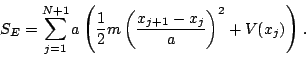
Taking $t_{i}=0$ , $x_{f}=x_{i}=x$ and $t_{f}=-iT$ with $T\rightarrow +\infty$ this can be used to compute the lowest energy levels and their wave functions

$\begin{displaymath} \vert\psi _{0}(x)\vert^{2}e^{-\frac{E_{0}}{\hbar }T}=\int [dx]e^{-\frac{1}{\hbar }S_{E}[x]} ,\qquad (T\rightarrow +\infty ).\end{displaymath}$

with $S_{E}[x]$ the Euclidean (for imaginary time) action

$\begin{displaymath} S_{E}[x]=\int ^{T}_{0}d\tau \left( \frac{1}{2}m\left( \frac{dx}{d\tau }\right) ^{2}+V(x)\right) .\end{displaymath}$

The path integral can be computed by discretizing the (Euclidean) time, then

$\begin{displaymath} \int [dx]e^{-\frac{1}{\hbar }S_{E}[x]}\sim \int ^{+\infty }_... ...e^{-\frac{1}{\hbar }S_{E}} ,\qquad (N\rightarrow \infty ) ,\end{displaymath}$

with $T=(N+1)a$ , and

$\begin{displaymath} S_{E}=\sum ^{N+1}_{j=1}a\left( \frac{1}{2}m\left( \frac{x_{j+1}-x_{j}}{a}\right) ^{2}+V(x_{j})\right) .\end{displaymath}$

We took $x_{0}=x_{N+1}=x$ in order to satisfy the boundary conditions $x_{0}=x=x_{i}=x_{f}$ . This integral can be computed numerically by using the Metropolis algorithm.

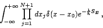
Although, in principle there is no integration on $x_{0}=x_{N+1}$ it is convenient to include it also in the integration since, due to the boundary conditions, all $x_{j}$ are completely equivalent. One does it by introducing an integration over $x_{0}$ of $\delta (x-x_{0})$

$\begin{displaymath} 1=\int _{-\infty }^{+\infty }dx_{0}\delta (x-x_{0})\end{displaymath}$

then we have

$\begin{displaymath} \int ^{+\infty }_{-\infty }\prod ^{N+1}_{j=1}dx_{j}\delta (x-x_{0})e^{-\frac{1}{\hbar }S_{E}} ,\end{displaymath}$

which can be understood as the expectation value of the function $\delta (x-x_{0})$ with the set $(x_{0},x_{1},\cdots ,x_{N})$ distributed according to the probability distribution $exp(-S_{E})$ . Thus, using Metropolis, we generate paths (sets of $x_{0},x_{1},\cdots ,x_{N}$ ) distributed according to $exp(-S_{E})$ . Then, we collect in a binned histogram the values of $x_{0}$ (but also the values of $x_{1},x_{2},\cdots x_{N}$ , since all the $x_{j}$ have the same distribution). This, with the appropriate normalization should give us the correct wave function squared $\vert\psi _{0}(x)\vert^{2}$ .

Once we have the wave function we can compute the expectation value of the Hamiltonian which should give us the energy of the lowest bound state, $E_{0}$ . For this we use the virial theorem

$\begin{displaymath} \frac{1}{2}m\langle v^{2}\rangle =\frac{1}{2}\langle xV^{\prime }(x)\rangle .\end{displaymath}$

For the potential we use

$\begin{displaymath} V(x)=\frac{1}{2}\mu x^{2}+\frac{1}{4}\lambda x^{4}+\theta (-\mu )\frac{\mu ^{2}}{4\lambda } ,\end{displaymath}$

where $\theta (x)$ is the step function and the last term ensures that the minimum of the potential is always zero. Thus, if $\lambda =0$ it is a harmonic oscillator with $\omega =\sqrt{\mu }$ ( $\mu$ must be positive). If $\lambda >0$ and $\mu <0$ the potential has two degenerate minima at $x=\pm v\equiv \pm \sqrt{-\mu /\lambda }$ .

The applet

The applet gives you in the upper panel the normalized wave function as a histogram (to be compared with a Gaussian which is the wave function of the harmonic oscillator ( $\lambda =0$ and $\mu =1$ ). The middle panel gives the energy $E_{0}$ as a function of the number of iterations. The lower panel gives a sample of the paths (as a function of time in units of $a$ ) that contribute more to the path integral formula. All expressions are for $\hbar =1$ and $m=1$ .

The button ``Potential'' opens a window with the potential and allows you to change it (clicking on the ``hand'' in the lower right corner). By changing it the simulation is restarted.

Yo can also ``pause'' and ``continue'' the simulation and print the panels.

All the simulations are performed for a lattice of $N=1000$ sites and with $a=0.1$ . The plots are updated only every $100$ iterations and the initial conditions for the iterations are also restarted randomly every $100$ iterations.

For ( $\lambda =0$ and $\mu >0$ ) you can see the nice Gaussian of the harmonic oscillator with $E_{0}=0.5\sqrt{\mu }$ .

For ( $\lambda >0$ and $\mu <0$ , try for instance $\lambda =2$ and $\mu =-10$ , ) there are two degenerate minima. Classically the particle stays in one of the two minima. In quantum mechanics, however, we can see that in the typical contributing paths the particle stays most of the time in one of the minima but from time to time it jumps to the other minimum (these are the so-called instantonic solutions) where it stays also some time. This allows the particle to stay half of the time in each of the two minima generating a wave function completely symmetric.

You will need the Java plugin (version 1.4 or above) to run the Path Integral applet (Click on the "Launch Applet" button to open it)

About this document ...

This document was generated using the LaTeX2HTML translator Version 2002 (1.62)

The command line arguments were:
latex2html -split 0 -nonavigation metro.tex

The translation was initiated by Arcadi Santamaria on 2004-12-09

Arcadi Santamaria 2004-12-09